In the past two parts, we saw that IV and RV are both mean-reverting. We also saw that we could use the edge generated from this mean-reverting behavior in our trading when we measure them using percentile (like we do in our option samurai option scanner). You can read part 2: Implied Volatility Backtest 2: Predicting RV Change here.
In this part, we want to do a quick test and see if there is a connection between them. Meaning – can we use IV rank to predict the RV, and can we use the RV rank to measure the IV.
Let’s frame the thesis into questions:
- Can we use extreme implied volatility to predict the future REAL volatility of an asset?
- Can we use extreme real volatility to predict the future IMPLIED volatility of an asset?
These are the questions we will explore in this article.
Quick recap:
[You can skip to the next part if you’ve read the previous articles.]
Implied Volatility Rank is a calculation used to give investors an idea of whether the IV of an asset is high or low at a glance. You can read more about it in our complete guide.
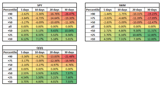
From the first article that compared IV rank and IV, we saw that we can expect the IV to decrease after a period of high IV rank and vise versa. Here is an example table from that article:

For example: In the table above, we can see that after IV rank was low (below 10 percentile), we saw IV rise 6.12% more than average in the following week).
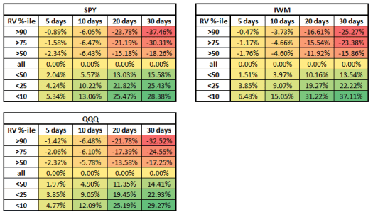
In the second article, we’ve also learned that the RV rank behaves similarly – after a period of low REAL volatility, we see an increase in real volatility and vise versa.

For example, after a high RV rank (90th percentile), we can see that the QQQ Real volatility decreased by 32.52% compared to regular volatility change in the following 30 trading days.
Comparing IV Rank to REAL Volatility
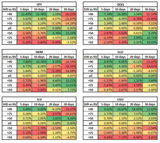
In the first part, we will see what happens to the REAL volatility when the implied volatility increases or decreases considerably. In the tables below, we can see a short-term link between implied volatility and real volatility: When IV increases, we can expect the RV to increase as well (in the next two weeks). However, after that, we can see a decrease in REAL volatility. This is also true for when IV decreases, but less extreme.

For example, when examining the SPY table, we can see that if implied volatility rises to the extreme (above 90%-ile), real volatility increases for the next five and ten days: 11.43% in the next week and 15.78% in the next two weeks, compared to ‘normal’ RV change. However, we can see that the real volatility decreases in the following month and 45 days. This is also in line with what we know from the IV behavior, and I suggest reading the first article linked above.
This also works the other way, but not as strong: we can see, for example, in the QQQ table, after implied volatility decreases, we see a reduction in real volatility for the next two weeks but an increase in volatility in the following 45 days. For example, after implied volatility is below 10%-ile, we can see a decrease in real volatility of 2.1% in a week and 3.34% in 2 weeks. These numbers are relative to the normal behavior of real volatility.
Comparing RV Rank to Implied Volatility
In this section, we will check how the REAL Volatility percentile impacts the future implied volatility.

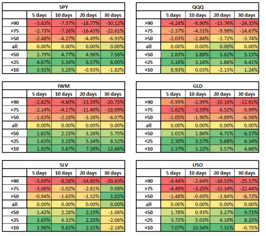
Since Real Volatility is a lagging indicator, we can see that the behavior or the RV percentile is similar to IV percentile’s behavior. After a high RV percentile, we can expect a decrease in IV, and vice versa: after a period of low RV, we can expect IV to rise.
For example, in SPY – we can see that after a 90%-ile RV Rank, we see a decrease in implied volatility of 3.63% in a week, 7.37% in 2 weeks, and 18.77% in a month.
This is also true for low values: After a low RV rank, we can expect an increase in implied volatility.
The edge here is weaker because real volatility is a lagging indicator, and the effect on implied volatility is not as strong. Still, we can use it to increase our advantage in the market and set up trades to help us.
If you wish to learn more, there is evidence that IV can also predict stock movement. A research done by researchers from Columbia and Georgetown universities showed some predictability. You can read it in our article: Trading Implied Volatility – Part 1 – Predicting stock movements
In conclusion:
IV is a predicting indicator – When it goes up fast, it usually means we can expect increased volatility to follow. The same goes when IV is extremely low – but it will be less violent. However, we know that IV will overshoot, so we can expect a reversion to the mean after the initial shock.
Similarly, we can use RV rank and set trades to benefit from the future increase or decrease in IV.
How to use in trading
Find trades with extreme IV Rank – In samurai, we have an IV rank filter as the default filter. You can set it up to filter for extreme values, such as: above 80% or below 20%, to find trades with extreme IV values. Once you find them – you can look for trend-following trades at the beginning and mean-reverting trades after a few days of extreme values.
Find trades with low RV rank for an extended period – You can add an RV percentile filter to help you find trades with extremely low RV values. This will also work for high RV values, but low RV values are advantageous in these market conditions. Since the RV behavior is slower, we recommend going to the analyze tab to see the RV chart and understand when it is the best time to enter trades. You can use this filter to help you trade limited-loss strategies that will benefit from an increase in IV, such as straddles, strangles, calendar spreads, and diagonals.
And if you want to check out one of the many ways in which you could profit from this theoretical approach, our example on a market plunge and VIX increase can help.

